Kevin Ummel (kevin.ummel@yale.edu)
About
⚠️ The fusionModel package provides an engine for generalized data fusion, implementing the statistical techniques described in Ummel et al. (2024). It is primarily intended for users looking to build their own custom fusion workflows using arbitrary datasets.
💡 Looking to analyze U.S. social survey microdata?
Practitioners interested in accessing and analyzing fused U.S. social survey microdata should instead use the purpose-built fusionACS R package, which is designed to streamline workflows across a variety of standard U.S. survey sources.
Overview
fusionModel enables variables unique to a “donor” dataset to be statistically simulated for (i.e. fused to) a “recipient” dataset. Variables common to both the donor and recipient are used to model and simulate the fused variables. The package provides a simple and efficient interface for general data fusion in R, leveraging state-of-the-art machine learning algorithms from Microsoft’s LightGBM framework. It also provides tools for analyzing synthetic/simulated data, calculating uncertainty, and validating fusion output.
fusionModel was developed to allow statistical integration of microdata from disparate social surveys. It is the data fusion workhorse underpinning the larger fusionACS data platform under development at the Socio-Spatial Climate Collaborative. In this context, fusionModel is used to fuse variables from a range of social surveys onto microdata from the American Community Survey, allowing for analysis and spatial resolution otherwise impossible.
Motivation
The desire to “fuse” or otherwise integrate independent datasets has a long history, dating to at least the early 1970’s (Ruggles and Ruggles 1974; Alter 1974). Social scientists have long recognized that large amounts of unconnected data are “out there” – usually concerning the characteristics of households and individuals (i.e. microdata) – which we would, ideally, like to integrate and analyze as a whole. This aim falls under the general heading of “Statistical Data Integration” (SDI) (Lewaa et al. 2021).
The most prominent examples of data fusion have involved administrative record linkage. This consists of exact matching or probabilistic linking of independent datasets, using observable information like social security numbers, names, or birth dates of individuals. Record linkage is the gold standard and can yield incredibly important insights and high levels of statistical confidence, as evidenced by the pioneering work of Raj Chetty and colleagues.
However, record linkage is rarely feasible for the kinds of microdata that most researchers use day-to-day (nevermind the difficulty of accessing administrative data). While the explosion of online tracking and social network data will undoubtedly offer new lines of analysis, for the time being, at least, social survey microdata remain indispensable. The challenge and promise recognized 50 years ago by Nancy and Richard Ruggles remains true today:
Unfortunately, no single microdata set contains all of the different kinds of information required for the problems which the economist wishes to analyze. Different microdata sets contain different kinds of information…A great deal of information is collected on a sample basis. Where two samples are involved the probability of the same individual appearing in both may be very small, so that exact matching is impossible. Other methods of combining the types of information contained in the two different samples into one microdata set will be required. (Ruggles and Ruggles 1974; 353-354)
Practitioners regularly impute or otherwise predict a variable or two from one dataset on to another. Piecemeal, ad hoc data fusion is a common necessity of quantitative research. Proper data fusion, on the other hand, seeks to systematically combine “two different samples into one microdata set”.
The size and nature of the samples involved and the intended analyses strongly influence the choice of data integration technique and the structure of the output. This has led to the relevant literature being both diverse and convoluted, as practitioners take on different data “setups” and objectives. In the context of fusionACS, we are interested in the following problem:
We have microdata from two independent surveys, A and B, that sample the same underlying population and time period (e.g. occupied U.S. households nationwide in 2018). We specify that A is the “recipient” dataset and B is the “donor”. The goal is to generate a new dataset, C, that has the original survey responses of A plus a realistic representation of how each respondent in A might have answered the questionnaire of survey B. To do this, we identify a set of common/shared variables X that both surveys solicit. We then attempt to fuse a set of variables unique to B – call them Z, the “fusion variables” – onto the original microdata of A, conditional on X.
Methodology
The fusion strategy implemented in the fusionModel package borrows and expands upon ideas from the statistical matching (D’Orazio et al. 2006), imputation (Little and Rubin 2019), and data synthesis (Drechsler 2011) literatures to create a flexible data fusion tool. It employs variable-k, conditional expectation matching that leverages high-performance gradient boosting algorithms. The package accommodates fusion of many variables, individually or in blocks, and efficient computation when the recipient is large relative to the donor.
Specifically, the goal was to create a data fusion tool that meets the following requirements:
- Accommodate donor and recipient datasets with divergent sample sizes
- Handle continuous, categorical, and semi-continuous (zero-inflated) variable types
- Ensure realistic values for fused variables
- Scale efficiently for larger datasets
- Fuse variables “one-by-one” or in “blocks”
- Employ a data modeling approach that:
- Makes no distributional assumptions (i.e. non-parametric)
- Automatically detects non-linear and interaction effects
- Automatically selects predictor variables from a potentially large set
- Ability to prevent overfitting (e.g. cross-validation)
Complete methodological details are available in Ummel et al. (2024).
Simple fusion
The package includes example microdata from the 2015 Residential Energy Consumption Survey (see ?recs for details). For real-world use cases, the donor and recipient data are typically independent and vary in sample size. For illustrative purposes, we will randomly split the recs microdata into separate “donor” and “recipient” datasets with an equal number of observations.
# Rows to use for donor dataset
d <- seq(from = 1, to = nrow(recs), by = 2)

# Create donor and recipient datasets
donor <- recs[d, c(2:16, 20:22)]
recipient <- recs[-d, 2:14]

# Specify fusion and shared/common predictor variables
predictor.vars <- names(recipient)
fusion.vars <- setdiff(names(donor), predictor.vars)
The recipient dataset contains 13 variables that are shared with donor. These shared “predictor” variables provide a statistical link between the two datasets. fusionModel exploits the information in these shared variables.
predictor.vars [1] "income" "age" "race" "education" "employment"
[6] "hh_size" "division" "urban_rural" "climate" "renter"
[11] "home_type" "year_built" "heat_type" There are 5 “fusion variables” unique to donor. These are the variables that will be fused to recipient. This includes a mix of continuous and categorical (factor) variables.
# The variables to be fused
sapply(donor[fusion.vars], class)$insulation
[1] "ordered" "factor"
$aircon
[1] "factor"
$square_feet
[1] "integer"
$electricity
[1] "integer"
$natural_gas
[1] "numeric"We create a fusion model using the train() function. The minimal usage is shown below. See ?train for additional function arguments and options. By default, this results in a “.fsn” (fusion) object being saved to “fusion_model.fsn” in the current working directory.
# Train a fusion model
fsn.model <- train(data = donor,
                   y = fusion.vars,
                   x = predictor.vars)
Using all available predictors for each fusion variable
- 5 fusion variables
- 13 predictor variables
- 2843 observations
-- Training step 1 of 5: insulation
-- Training step 2 of 5: aircon
-- Training step 3 of 5: square_feet
-- R-squared of cluster means: 0.98
-- Number of neighbors in each cluster:
Min. 1st Qu. Median Mean 3rd Qu. Max.
10.0 27.0 94.5 178.0 353.2 498.0
-- Training step 4 of 5: electricity
-- R-squared of cluster means: 0.974
-- Number of neighbors in each cluster:
Min. 1st Qu. Median Mean 3rd Qu. Max.
10.0 37.0 105.0 177.8 327.0 497.0
-- Training step 5 of 5: natural_gas
-- R-squared of cluster means: 0.959
-- Number of neighbors in each cluster:
Min. 1st Qu. Median Mean 3rd Qu. Max.
10.0 43.0 133.0 192.4 344.0 498.0
Fusion model saved to:
/home/kevin/Documents/Projects/fusionModel/fusion_model.fsn
Total processing time: 6.45 secsTo fuse variables to recipient, we simply pass the recipient data and path of the .fsn model to the fuse() function. Each variable specified in fusion.vars is fused in the order provided. By default, fuse() generates a single implicate (version) of synthetic outcomes. Later, we’ll work with multiple implicates to perform proper analysis and uncertainty estimation.
# Fuse 'fusion.vars' to the recipient
sim <- fuse(data = recipient,
            fsn = fsn.model)
- 5 fusion variables
- 13 initial predictor variables
- 2843 observations
- Available memory: 40.1 GB
- Implicates: 1
-- Fusion step 1 of 5: insulation
- Predicting LightGBM models
- Simulating fused values
-- Fusion step 2 of 5: aircon
- Predicting LightGBM models
- Simulating fused values
-- Fusion step 3 of 5: square_feet
- Predicting LightGBM models
- Simulating fused values
-- Fusion step 4 of 5: electricity
- Predicting LightGBM models
- Simulating fused values
-- Fusion step 5 of 5: natural_gas
- Predicting LightGBM models
- Simulating fused values
Total processing time: 0.729 secsLet’s look at the the recipient dataset’s fused/simulated variables. Note that your results will look different, because each call to fuse() generates a unique, probabilistic set of outcomes.
head(sim)Key: <M>
M insulation aircon
<int> <ord> <fctr>
1: 1 Adequately insulated Individual window/wall or portable units
2: 1 Adequately insulated Central air conditioning system
3: 1 Poorly insulated Individual window/wall or portable units
4: 1 Adequately insulated Central air conditioning system
5: 1 Adequately insulated Central air conditioning system
6: 1 Adequately insulated Central air conditioning system
square_feet electricity natural_gas
<int> <int> <num>
1: 1548 14670 0.0
2: 2460 15160 179.5
3: 761 2200 0.0
4: 2160 11220 1150.0
5: 4210 21300 0.0
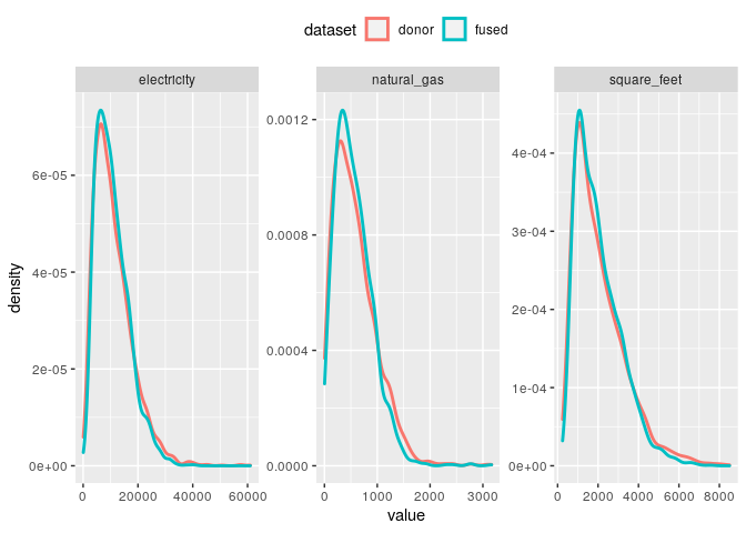
6: 1323 8420 220.0We can do some quick sanity checks to compare the distribution of the fusion variables in donor with those in sim. This, at least, confirms that the fusion output is not obviously wrong. Later, we’ll perform a formal internal validation exercise using multiple implicates.
sim <- data.frame(sim)

# Compare means of the continuous variables
cbind(donor = colMeans(donor[fusion.vars[3:5]]), sim = colMeans(sim[fusion.vars[3:5]]))
donor sim
square_feet 2070.784 2075.9100
electricity 10994.517 10795.8692
natural_gas 338.154 340.0952
# Compare frequencies of categorical variable classes
cbind(donor = table(donor$insulation), sim = table(sim$insulation))
donor sim
Not insulated 40 35
Poorly insulated 459 428
Adequately insulated 1401 1401
Well insulated 943 979 donor sim
Central air conditioning system 1788 1746
Individual window/wall or portable units 545 532
Both a central system and individual units 125 148
No air conditioning 385 417And we can look at kernel density plots of the non-zero values for the continuous variables to see if the univariate distributions in donor are generally similar in sim.
Advanced fusion
When working with datasets containing numerous or potentially correlated/collinear variables, prepXY() provides an automated way to screen predictors and optimize fusion variable ordering before model training. It pairs an initial rank-correlation screening step with LASSO regularization (via glmnet) to filter out weak predictors and then determines a preferred fusion sequence among the fusion variables.
Using the donor microdata and variable sets defined earlier:
# Screen predictors and determine optimal target fusion order
xy_prep <- prepXY(data = donor,
                  y = fusion.vars,
                  x = predictor.vars)
Identifying 'x' predictors passing Spearman correlation threshold (cor_thresh = 0.05)...
Fitting full LASSO models for each 'y'...
Iteratively constructing preferred fusion order...
- Retained 13 of 13 potential predictor variables
- prepXY() completed in 0.355 secsBecause we have a relatively small number of highly-relevant predictor variables in this example, prepXY() retained all of the predictor.vars. The output of prepXY() can be passed directly to train(). This is especially helpful when automating fusion using larger donor datasets.
# Train a basic fusion model using the prepXY output
fsn.model <- train(data = donor,
                   y = xy_prep$y,
                   x = xy_prep$x)
Using specified set of predictors for each fusion variable
- 5 fusion variables
- 13 predictor variables
- 2843 observations
-- Training step 1 of 5: insulation
-- Training step 2 of 5: aircon
-- Training step 3 of 5: square_feet
-- R-squared of cluster means: 0.97
-- Number of neighbors in each cluster:
Min. 1st Qu. Median Mean 3rd Qu. Max.
10.0 33.0 98.0 170.8 291.5 497.0
-- Training step 4 of 5: natural_gas
-- R-squared of cluster means: 0.948
-- Number of neighbors in each cluster:
Min. 1st Qu. Median Mean 3rd Qu. Max.
10.0 56.0 175.0 229.1 432.0 498.0
-- Training step 5 of 5: electricity
-- R-squared of cluster means: 0.944
-- Number of neighbors in each cluster:
Min. 1st Qu. Median Mean 3rd Qu. Max.
10.0 38.0 108.0 184.0 344.5 497.0
Fusion model saved to:
/home/kevin/Documents/Projects/fusionModel/fusion_model.fsn
Total processing time: 4.58 secsFor a more sophistiaced call to train(), we specify a set of hyperparameters to search over when training each LightGBM gradient boosting model (see ?train for details). The hyperparameters can be used to tune the underlying GBM models for better cross-validated performance. We also set nfolds = 10 (default is 5) to indicate the number of cross-validation folds to use. Since this requires additional computation, the cores argument is used to enable parallel processing.
# Train a fusion model with variable blocks
fsn.model <- train(data = donor,
                   y = xy_prep$y,
                   x = xy_prep$x,
                   nfolds = 10,
                   hyper = list(boosting = c("gbdt", "goss"),
                                num_leaves = c(10, 30),
                                feature_fraction = c(0.7, 0.9)),
                   cores = 2)
Using specified set of predictors for each fusion variable
- 5 fusion variables
- 13 predictor variables
- 2843 observations
Using OpenMP multithreading within LightGBM (2 cores)
-- Training step 1 of 5: insulation
-- Training step 2 of 5: aircon
-- Training step 3 of 5: square_feet
-- R-squared of cluster means: 0.938
-- Number of neighbors in each cluster:
Min. 1st Qu. Median Mean 3rd Qu. Max.
10.0 37.0 127.0 204.3 405.5 498.0
-- Training step 4 of 5: natural_gas
-- R-squared of cluster means: 0.962
-- Number of neighbors in each cluster:
Min. 1st Qu. Median Mean 3rd Qu. Max.
10.0 43.0 120.0 182.1 301.0 498.0
-- Training step 5 of 5: electricity
-- R-squared of cluster means: 0.949
-- Number of neighbors in each cluster:
Min. 1st Qu. Median Mean 3rd Qu. Max.
10.0 34.0 92.0 169.5 287.0 495.0
Fusion model saved to:
/home/kevin/Documents/Projects/fusionModel/fusion_model.fsn
Total processing time: 20.9 secsWe generally want to create multiple versions of the simulated fusion variables – called implicates – in order to reduce bias in point estimates and calculate associated uncertainty. We can do this using the M argument within fuse(). Here we generate 10 implicates; i.e. 10 unique, probabilistic representations of what the recipient records might look like with respect to the fusion variables.
# Fuse multiple implicates to the recipient
sim10 <- fuse(data = recipient,
              fsn = fsn.model,
              M = 10)
- 5 fusion variables
- 13 initial predictor variables
- 2843 observations
- Available memory: 39.8 GB
- Implicates: 10
-- Fusion step 1 of 5: insulation
- Predicting LightGBM models
- Simulating fused values
-- Fusion step 2 of 5: aircon
- Predicting LightGBM models
- Simulating fused values
-- Fusion step 3 of 5: square_feet
- Predicting LightGBM models
- Simulating fused values
-- Fusion step 4 of 5: natural_gas
- Predicting LightGBM models
- Simulating fused values
-- Fusion step 5 of 5: electricity
- Predicting LightGBM models
- Simulating fused values
Total processing time: 1.37 secsNote that each implicate in sim10 is identified by the “M” variable/column.
head(sim10)Key: <M>
M insulation aircon
<int> <ord> <fctr>
1: 1 Adequately insulated No air conditioning
2: 1 Adequately insulated Central air conditioning system
3: 1 Adequately insulated Central air conditioning system
4: 1 Adequately insulated Individual window/wall or portable units
5: 1 Well insulated No air conditioning
6: 1 Poorly insulated No air conditioning
square_feet natural_gas electricity
<int> <num> <int>
1: 1204 371 3610
2: 2215 689 7170
3: 952 67 6150
4: 1106 726 22200
5: 3935 923 7630
6: 1073 518 1480
table(sim10$M)Analyzing fused data
[!IMPORTANT] The
analyze()function in thefusionModelpackage documents and implements the point estimate and variance estimation methodology used in Ummel et al. (2024). A newer, improved analysis approach has since been introduced in thefusionACSpackage (fusionACS Methods). Whileanalyze()is retained for legacy support and replication purposes, users are encouraged to review the updatedfusionACSworkflow for improved analysis techniques.
The fused values are inherently probabilistic, reflecting uncertainty in the underlying statistical models. Multiple implicates are needed to calculate unbiased point estimates and associated uncertainty for any particular analysis of the data. In general, more implicates is preferable but requires more computation.
Since proper analysis of multiple implicates can be rather cumbersome – both from a coding and mathematical standpoint – the analyze() function provides a convenient way to calculate point estimates and associated uncertainty for common analyses. Potential analyses currently include variable means, proportions, sums, counts, and medians, (optionally) calculated for population subgroups.
For example, to calculate the mean value of the “electricity” variable across all observations in the recipient dataset, we do the following.
ℹ Using 10 implicates

ℹ Assuming uniform sample weights

✔ Total processing time: 0.0227 secs

       N           y  level   type      est      moe
   <int>      <char> <lgcl> <char>    <num>    <num>
1:  2843 electricity     NA   mean 11149.65 302.5612
When the response variable is categorical, analyze() automatically returns the proportions associated with each factor level.
ℹ Using 10 implicates

ℹ Assuming uniform sample weights

✔ Total processing time: 0.0584 secs

       N      y                                      level       type
   <int> <char>                                     <char>     <char>
1:  2843 aircon            Central air conditioning system proportion
2:  2843 aircon   Individual window/wall or portable units proportion
3:  2843 aircon Both a central system and individual units proportion
4:  2843 aircon                        No air conditioning proportion
          est         moe
        <num>       <num>
1: 0.62296870 0.022589716
2: 0.19704537 0.017080786
3: 0.04386212 0.008929643
4: 0.13612381 0.015763985
If we want to perform an analysis across subsets of the recipient population – for example, calculate the mean value of “electricity” by household “income” – we can use the by and static arguments. We see that mean electricity consumption increases with household income.
ℹ Using 10 implicates

ℹ Assuming uniform sample weights

✔ Total processing time: 0.0246 secs

                 income     N           y  level   type       est       moe
                  <ord> <int>      <char> <lgcl> <char>     <num>     <num>
1:    Less than $20,000   471 electricity     NA   mean  9046.579  527.2344
2:    $20,000 - $39,999   645 electricity     NA   mean 10062.808  539.6401
3:    $40,000 - $59,999   464 electricity     NA   mean 10830.042  736.3983
4:   $60,000 to $79,999   372 electricity     NA   mean 11545.838  693.1825
5:   $80,000 to $99,999   248 electricity     NA   mean 12117.840  813.2068
6: $100,000 to $119,999   222 electricity     NA   mean 12623.509 1061.2703
7: $120,000 to $139,999   119 electricity     NA   mean 13272.992 1264.6678
8:     $140,000 or more   302 electricity     NA   mean 14038.658  985.1132
It is also possible to do multiple kinds of analyses in a single call to analyze(). For example, the following call calculates the mean value of “natural_gas” and “square_feet”, the median value of “square_feet”, and the sum of “electricity” (i.e. total consumption) and “insulation” (i.e. total count of each level). All of these estimates are calculated for each population subgroup defined by the intersection of “race” and “urban_rural” status.
result <- analyze(x = list(mean = c("natural_gas", "square_feet"),
                           median = "square_feet",
                           sum = c("electricity", "insulation")),
                  implicates = sim10,
                  static = recipient,
by = c("race", "urban_rural"))We can then (for example) isolate the results for white households in rural areas. Notice that the mean estimate of “square_feet” exceeds the median, reflecting the skewed distribution.
subset(result, race == "White" & urban_rural == "Rural") race urban_rural N y level type
<fctr> <fctr> <int> <char> <char> <char>
1: White Rural 503 electricity <NA> sum
2: White Rural 503 insulation Not insulated count
3: White Rural 503 insulation Poorly insulated count
4: White Rural 503 insulation Adequately insulated count
5: White Rural 503 insulation Well insulated count
6: White Rural 503 natural_gas <NA> mean
7: White Rural 503 square_feet <NA> mean
8: White Rural 503 square_feet <NA> median
est moe
<num> <num>
1: 6879414.6000 458249.58083
2: 5.7000 4.87618
3: 72.4000 15.46669
4: 218.0000 22.94028
5: 206.9000 24.80348
6: 221.5125 50.80821
7: 2313.7581 173.23956
8: 2033.5000 221.23380More complicated analyses can be performed using the custom fun argument to analyze(). See the Examples section of ?analyze.
Validating fusion models
The validate() function provides a convenient way to perform internal validation tests on synthetic variables that have been fused back onto the original donor data. This allows us to assess the quality of the underlying fusion model; it is analogous to assessing model skill by comparing predictions to the observed training data.
validate() compares analytical results derived using the multiple-implicate fusion output with those derived using the original donor microdata. By performing analyses on population subsets of varying size, validate() estimates how the synthetic variables perform for analyses of varying difficulty/complexity. It computes fusion variable means and proportions for subsets of the full sample – separately for both the observed and fused data – and then compares the results.
First, we fuse multiple implicates of the fusion.vars using the original donor data – not the recipient data, as we did previously.
sim <- fuse(data = donor,
            fsn = fsn.model,
            M = 40)
- 5 fusion variables
- 13 initial predictor variables
- 2843 observations
- Available memory: 39.8 GB
- Implicates: 40
-- Fusion step 1 of 5: insulation
- Predicting LightGBM models
- Simulating fused values
-- Fusion step 2 of 5: aircon
- Predicting LightGBM models
- Simulating fused values
-- Fusion step 3 of 5: square_feet
- Predicting LightGBM models
- Simulating fused values
-- Fusion step 4 of 5: natural_gas
- Predicting LightGBM models
- Simulating fused values
-- Fusion step 5 of 5: electricity
- Predicting LightGBM models
- Simulating fused values
Total processing time: 2.93 secsNext, we pass the sim results to validate(). The argument subset_vars specifies that we want the validation exercise to compare observed (donor) and simulated point estimates across population subsets defined by “income”, “age”, “race”, and “education”. See ?validate for more details.
valid <- validate(observed = donor,
                  implicates = sim,
                  subset_vars = c("income", "age", "race", "education"))
Assuming uniform sample weights
One-hot encoding categorical fusion variables
Correlation between observed and fused values:
Min. 1st Qu. Median Mean 3rd Qu. Max.
0.037 0.060 0.068 0.130 0.163 0.389
Processing validation analyses for 5 fusion variables
Performed 1419 analyses across 129 subsets
Smoothing validation metrics
Average smoothed performance metrics across subset range:
y est vad moe
1 aircon 0.04633 0.614 1.42
2 electricity 0.01572 0.747 1.22
3 insulation 0.04367 0.351 1.43
4 natural_gas 0.02677 0.778 1.34
5 square_feet 0.00786 0.895 1.31
Creating ggplot2 graphics
Total processing time: 2.38 secsThe validate() output includes ggplot2 graphics that helpfully summarize the validation results. For example, the plot below shows how the observed and simulated point estimates compare, using median absolute percent error as the performance metric. We see that the synthetic data do a very good job reproducing the point estimates for all fusion variables when the population subset in question is reasonably large. For smaller subsets – i.e. more difficult analyses due to small sample size – “square_feet”, “natural_gas”, and “electricity” remain well modeled, but the error increases more rapidly for “aircon” and “insulation”. This information is useful for understanding what kind of reliability we can expect for particular variables and types of analyses, given the underlying fusion model and data.
valid$plots$est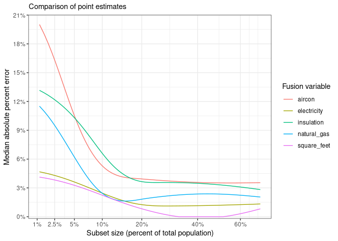
Happy fusing!